Session Info
paratbc
Status:
Completed
Progress
2 / 2 steps completed
Quick Actions
Dataset Overview
7642
Rows2
ColumnsColumn Types
Column Information
| Column | Type | Non-Null Count | Missing % | Unique Values |
|---|---|---|---|---|
| Id | int64 | 7642 | 0% | 7642 |
| DateCreated | datetime64[ns] | 7642 | 0% | 7641 |
Generated SQL Query
Query length: 141
SELECT TOP 25000
    t.Id,
    t.DateCreated
FROM Requests t
WHERE t.DateCreated >= DATEADD(MONTH, -6, GETDATE())
ORDER BY t.DateCreated DESCAsk Your Question
Analysis History
Select for context:
Analysis 1
Descriptive statistics on the analysis type distribution in time and relative numbers.
2026-02-13 17:05:25 • 16 files
Debug: Found 16 generated files (1 scripts)
Generated Visualizations
Generated visualization
plot_04_hourly_distribution.png
Generated visualization
plot_03_day_of_week_distribution.png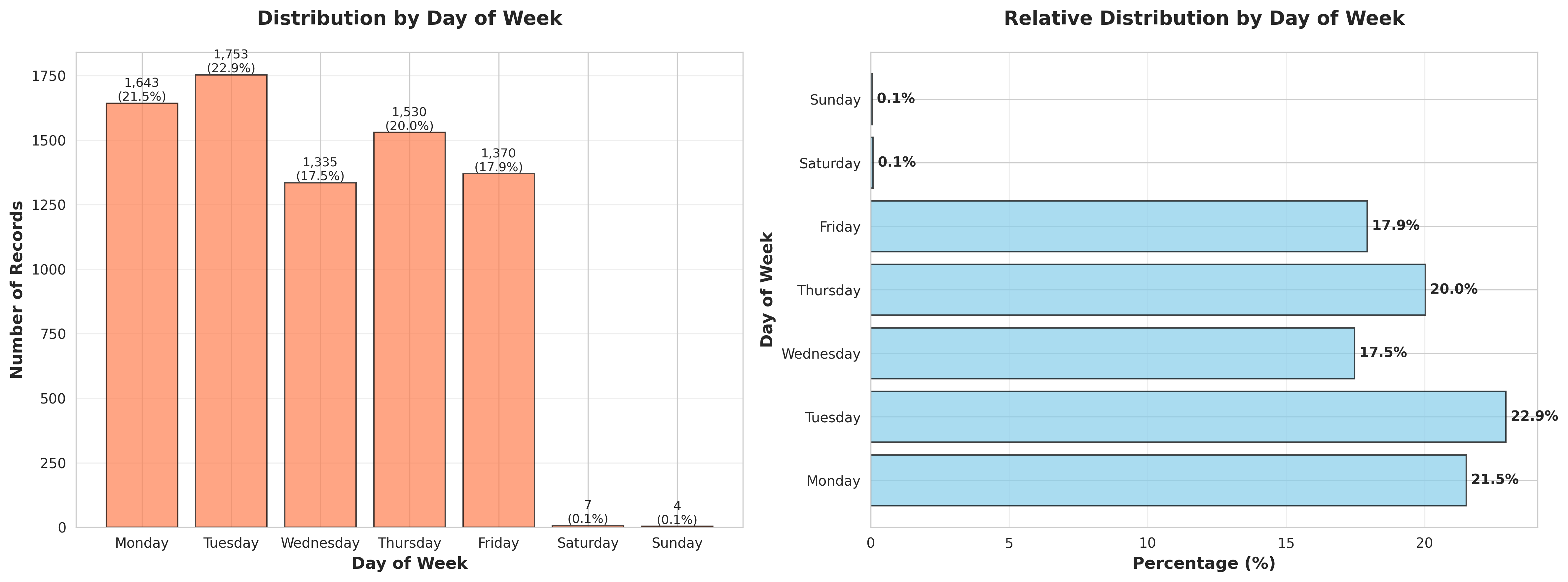
Generated visualization
plot_06_trend_analysis.png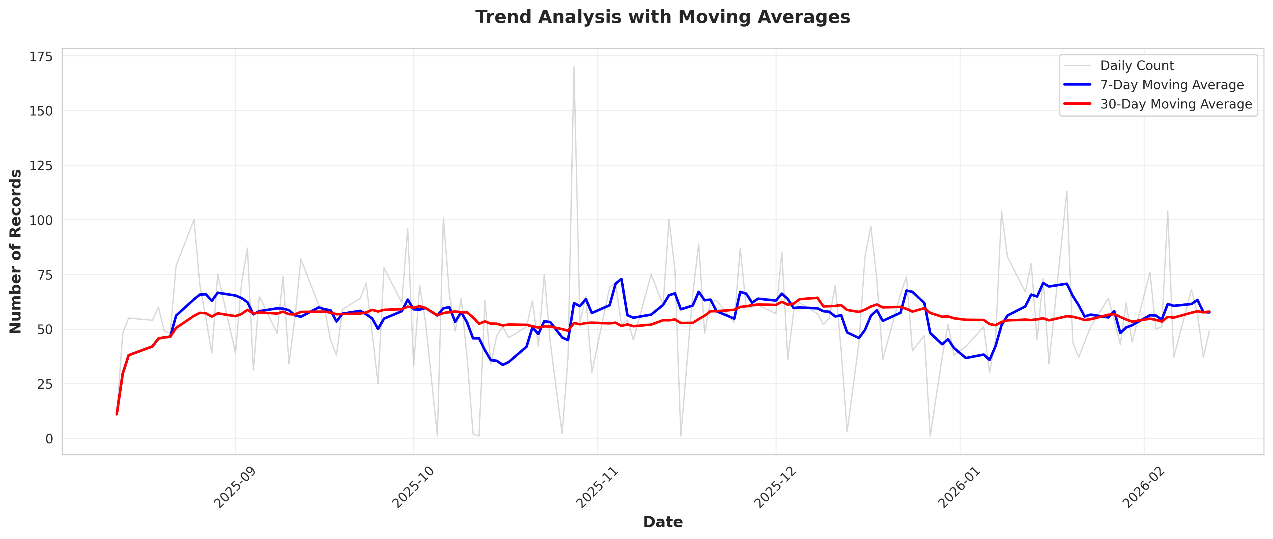
Generated visualization
plot_05_day_hour_heatmap.png
Generated visualization
plot_01_daily_time_series.png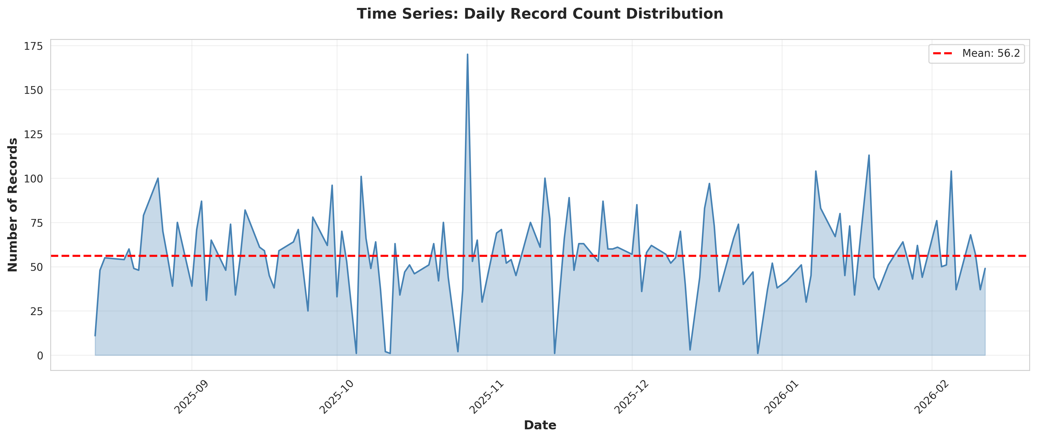
Generated visualization
plot_02_monthly_distribution.png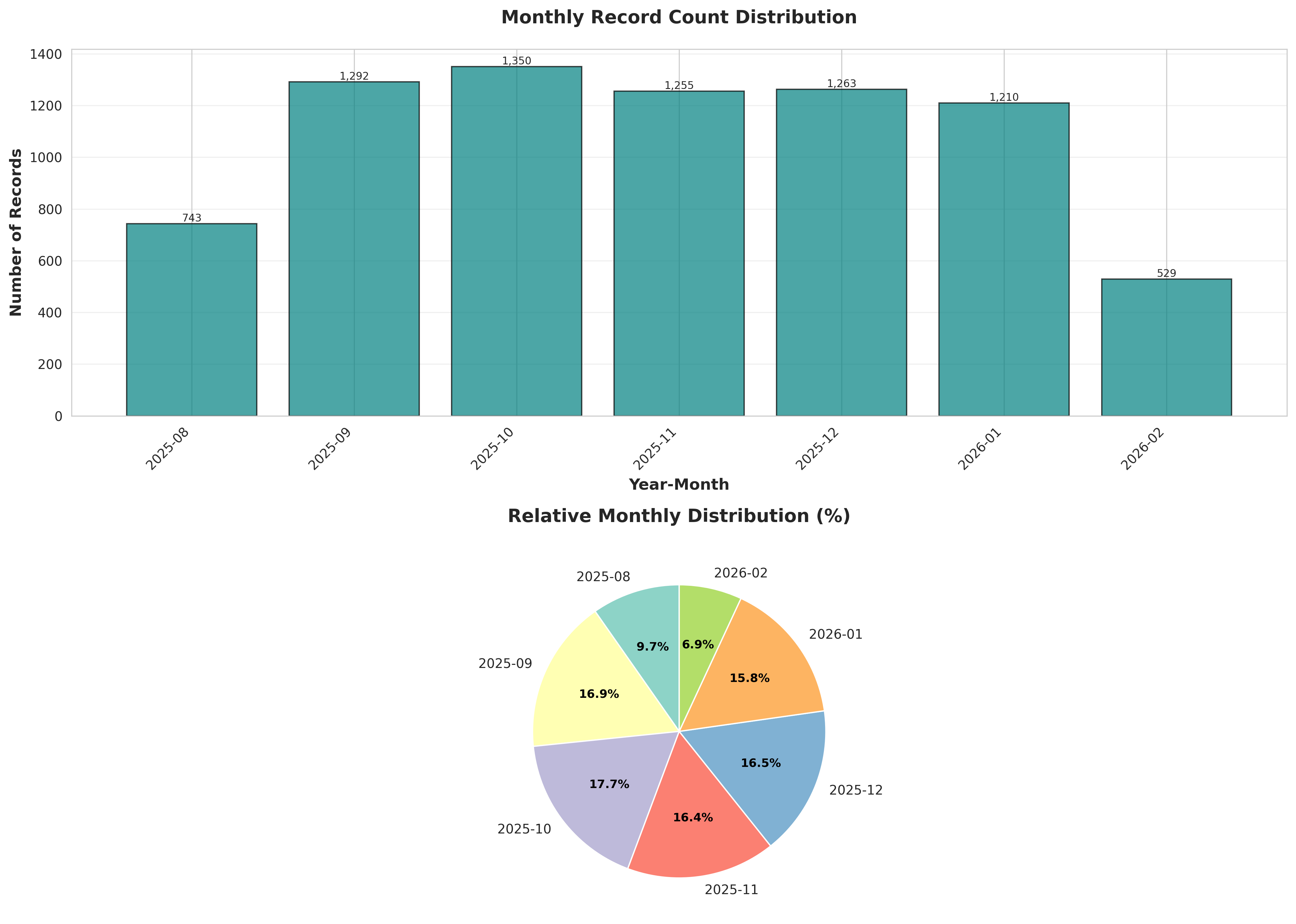
Generated Tables
Data table or results
table_02_monthly_distribution.csvYear-Month,Count,Percentage (%),Cumulative (%) 2025-08,743,9.722585710546976,9.722585710546976 2025-09,1292,16.90656896100497,26.629154671551948 2025-10,1350,17.665532583093434,44.29468725464538 2025-11,1255,16.4224025124313,60.717089767076686 2025-12,1263,16.527087149960742,77.24417691703744 2026-01,1210,15.833551426328185,93.07772834336562 2026-02,529,6.922271656634389,100.00000000000001
Data table or results
table_06_overall_statistics.csvStatistic,Value Total Records,"7,642" Unique Dates,136 Date Range (days),183 Average Records per Day,56.19 Median Records per Day,54.50 Std Dev Records per Day,24.14 Coefficient of Variation (%),42.97 Min Records per Day,1 Max Records per Day,170 Records per Hour (avg),318.42 Most Common Hour,09:00 Most Common Day,Tuesday
Data table or results
table_05_time_period_distribution.csvTime Period,Count,Percentage Afternoon (12-17),3920,51.295472389426855 Evening (18-23),42,0.5495943470295734 Morning (6-11),3680,48.154933263543576
Data table or results
table_01_temporal_summary_statistics.csvMetric,Value Mean Daily Count,56.19117647058823 Median Daily Count,54.5 Std Dev Daily Count,24.142943054781146 Min Daily Count,1.0 Max Daily Count,170.0 Total Days,136.0 Days with Activity,136.0 Average per Active Day,56.19117647058823
Data table or results
table_04_hourly_distribution.csvHour,Count,Percentage (%),Time Period 6,11,0.1439413766029835,Morning (6-11) 7,102,1.3347291285003926,Morning (6-11) 8,951,12.444386286312485,Morning (6-11) 9,1118,14.629678094739598,Morning (6-11) 10,793,10.376864695105994,Morning (6-11) 11,705,9.225333682282125,Morning (6-11) 12,664,8.688824914943732,Afternoon (12-17) 13,639,8.361685422664223,Afternoon (12-17) 14,921,12.051818895577075,Afternoon (12-17) 15,903,11.816278461135827,Afternoon (12-17) 16,661,8.649568175870192,Afternoon (12-17) 17,1...
Data table or results
input_data.csvId,DateCreated 65634,2026-02-12 12:33:20 65633,2026-02-12 12:32:57 65632,2026-02-12 12:30:35 65631,2026-02-12 12:23:35 65630,2026-02-12 12:20:41 65629,2026-02-12 12:05:32 65628,2026-02-12 12:05:18 65627,2026-02-12 12:00:52 65626,2026-02-12 11:57:50 65625,2026-02-12 11:54:57 65624,2026-02-12 11:49:43 65623,2026-02-12 11:45:19 65622,2026-02-12 11:42:00 65621,2026-02-12 11:39:57 65620,2026-02-12 11:34:14 65619,2026-02-12 11:27:51 65618,2026-02-12 11:22:19 65617,2026-02-12 11:18:09 65616,2026-02-12 ...
Data table or results
table_03_day_of_week_distribution.csvDay of Week,Count,Percentage (%) Monday,1643,21.499607432609263 Tuesday,1753,22.9390211986391 Wednesday,1335,17.469248887725726 Thursday,1530,20.02093692750589 Friday,1370,17.927244176917036 Saturday,7,0.09159905783826224 Sunday,4,0.05234231876472127
Analysis Conclusions
Analysis conclusions and insights
conclusions.txt
======================================================================
STATISTICAL ANALYSIS REPORT
Descriptive Statistics on Analysis Type Distribution in Time
======================================================================
Analysis Date: 2026-02-12 11:44:39
Total Records: 7,642
Date Range: 2025-08-12 13:35:14 to 2026-02-12 12:33:20
Time Span: 183 days
----------------------------------------------------------------------
1. OVERALL TEMPORAL DISTRIBUTION
----------------------------------------------------------------------
Mean daily count: 56.19
Median daily count: 54.50
Standard deviation: 24.14
Range: 1 to 170
----------------------------------------------------------------------
2. MONTHLY DISTRIBUTION
----------------------------------------------------------------------
Number of months: 7
Average records per month: 1091.71
Most active month: 2025-10 (1,350 records)
Least active month: 2026-02 (529 records)
----------------------------------------------------------------------
3. DAY OF WEEK DISTRIBUTION
----------------------------------------------------------------------
Monday: 1,643 records (21.50%)
Tuesday: 1,753 records (22.94%)
Wednesday: 1,335 records (17.47%)
Thursday: 1,530 records (20.02%)
Friday: 1,370 records (17.93%)
Saturday: 7 records (0.09%)
Sunday: 4 records (0.05%)
Most active day: Tuesday
Least active day: Sunday
----------------------------------------------------------------------
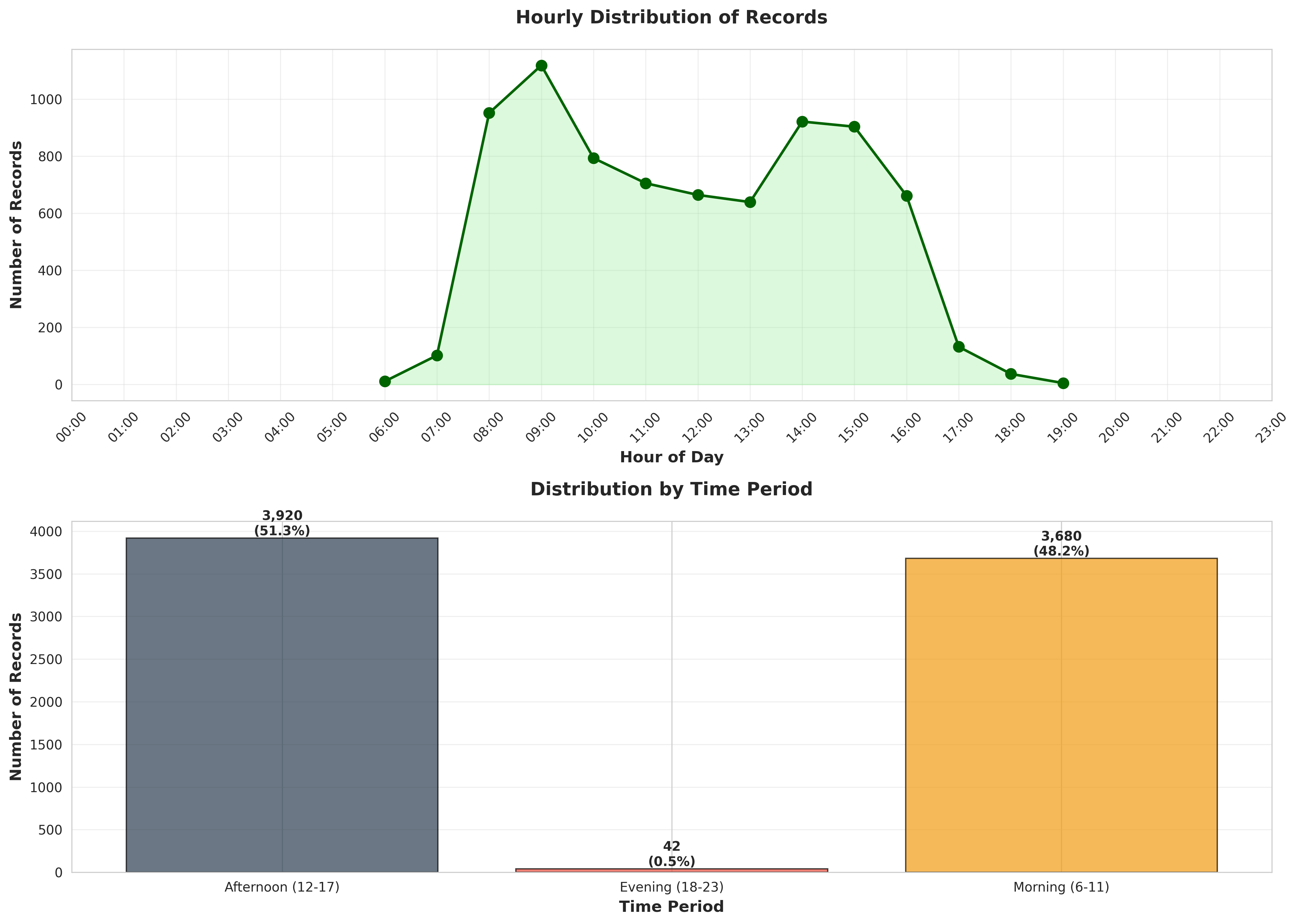
4. HOURLY DISTRIBUTION
----------------------------------------------------------------------
Peak hour: 09:00 (1,118 records)
Lowest hour: 19:00 (5 records)
Time Period Distribution:
Afternoon (12-17): 3,920 records (51.30%)
Evening (18-23): 42 records (0.55%)
Morning (6-11): 3,680 records (48.15%)
----------------------------------------------------------------------
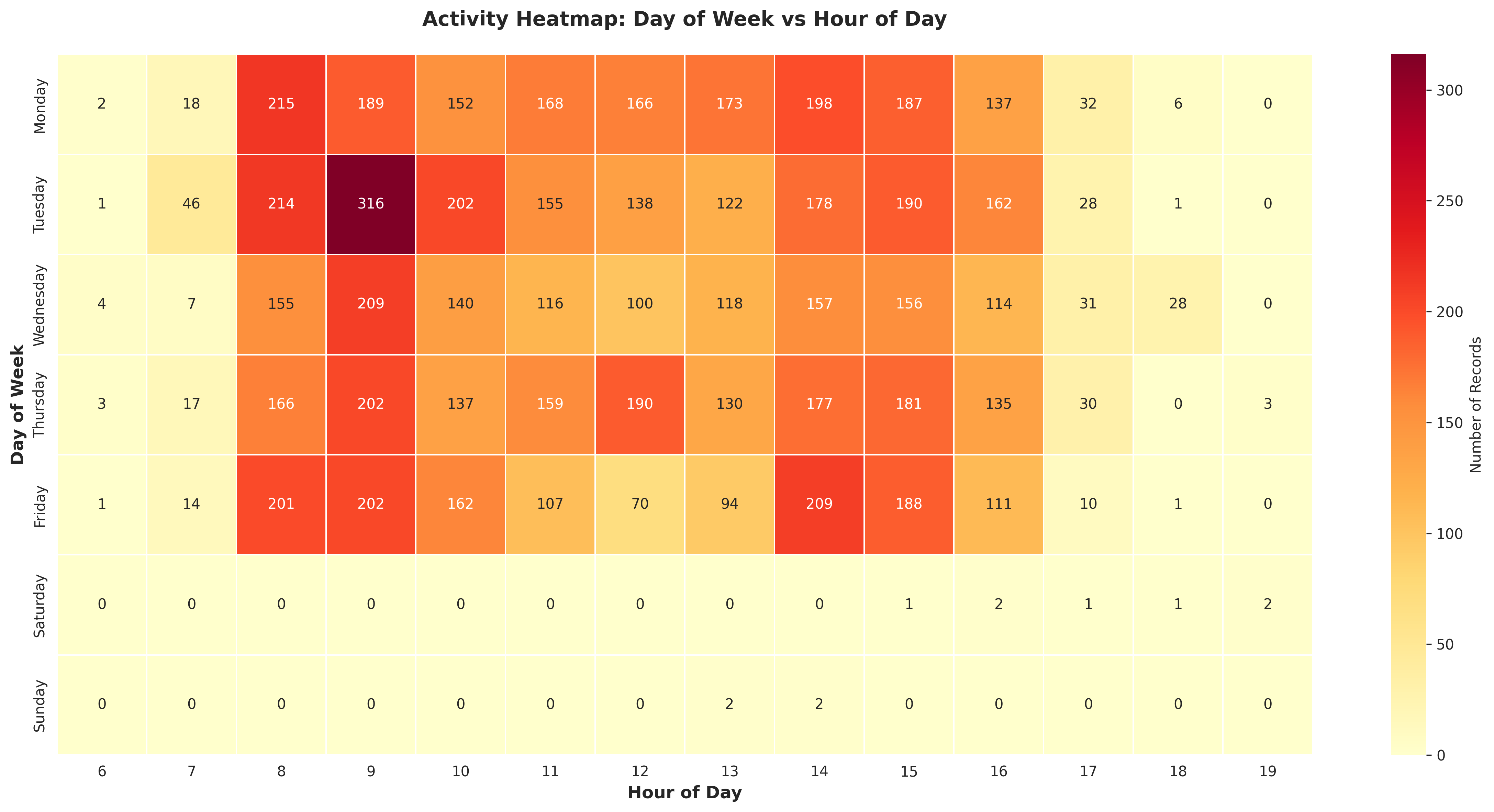
5. DAY-HOUR PATTERN ANALYSIS
----------------------------------------------------------------------
Peak activity: Tuesday at 09:00 (316 records)
--------------------------
STATISTICAL ANALYSIS REPORT
Descriptive Statistics on Analysis Type Distribution in Time
======================================================================
Analysis Date: 2026-02-12 11:44:39
Total Records: 7,642
Date Range: 2025-08-12 13:35:14 to 2026-02-12 12:33:20
Time Span: 183 days
----------------------------------------------------------------------
1. OVERALL TEMPORAL DISTRIBUTION
----------------------------------------------------------------------
Mean daily count: 56.19
Median daily count: 54.50
Standard deviation: 24.14
Range: 1 to 170
----------------------------------------------------------------------
2. MONTHLY DISTRIBUTION
----------------------------------------------------------------------
Number of months: 7
Average records per month: 1091.71
Most active month: 2025-10 (1,350 records)
Least active month: 2026-02 (529 records)
----------------------------------------------------------------------
3. DAY OF WEEK DISTRIBUTION
----------------------------------------------------------------------
Monday: 1,643 records (21.50%)
Tuesday: 1,753 records (22.94%)
Wednesday: 1,335 records (17.47%)
Thursday: 1,530 records (20.02%)
Friday: 1,370 records (17.93%)
Saturday: 7 records (0.09%)
Sunday: 4 records (0.05%)
Most active day: Tuesday
Least active day: Sunday
----------------------------------------------------------------------
4. HOURLY DISTRIBUTION
----------------------------------------------------------------------
Peak hour: 09:00 (1,118 records)
Lowest hour: 19:00 (5 records)
Time Period Distribution:
Afternoon (12-17): 3,920 records (51.30%)
Evening (18-23): 42 records (0.55%)
Morning (6-11): 3,680 records (48.15%)
----------------------------------------------------------------------
5. DAY-HOUR PATTERN ANALYSIS
----------------------------------------------------------------------
Peak activity: Tuesday at 09:00 (316 records)
--------------------------
Generated Scripts
Generated Python analysis script
analysis.py
Content length: 23274
#!/usr/bin/env python3
"""
Statistical Analysis Script
Generated by SmartStat Agent
Query: Descriptive statistics on the analysis type distribution in time and relative numbers.
Generated: 2026-02-12T11:41:20.153787
"""

import pandas as pd
import numpy as np
import matplotlib
matplotlib.use('Agg')
import matplotlib.pyplot as plt
import seaborn as sns
from scipy import stats
from datetime import datetime
import warnings
warnings.filterwarnings('ignore')

# Set style for better-looking plots
sns.set_style("whitegrid")
plt.rcParams['figure.figsize'] = (12, 6)
plt.rcParams['font.size'] = 10

def main():
    print("Starting statistical analysis...")
    print("Query: Descriptive statistics on the analysis type distribution in time and relative numbers.")

    # Load data
    try:
        df = pd.read_csv('input_data.csv')
        print(f"Data loaded successfully: {df.shape}")
    except Exception as e:
        print(f"Error loading data: {e}")
        return

    # Data validation and preprocessing
    print("\n" + "="*60)
    print("DATA PREPROCESSING")
    print("="*60)

    try:
        # Convert DateCreated to datetime
        df['DateCreated'] = pd.to_datetime(df['DateCreated'])
        print("✓ DateCreated converted to datetime format")

        # Extract temporal features
        df['Year'] = df['DateCreated'].dt.year
        df['Month'] = df['DateCreated'].dt.month
        df['YearMonth'] = df['DateCreated'].dt.to_period('M')
        df['Week'] = df['DateCreated'].dt.isocalendar().week
        df['DayOfWeek'] = df['DateCreated'].dt.dayofweek
        df['DayName'] = df['DateCreated'].dt.day_name()
        df['Hour'] = df['DateCreated'].dt.hour
        df['Date'] = df['DateCreated'].dt.date

        print("✓ Temporal features extracted")

    except Exception as e:
        print(f"Error in preprocessing: {e}")
        return

    # Initialize conclusions file
    conclusions = []
    conclusions.append("="*70)
    conclusions.append("STATISTICAL ANALYSIS REPORT")
    conclusions.append("Descriptive Statistics on Analysis Type Distribution in Time")
    conclusions.append("="*70)
    conclusions.append(f"\nAnalysis Date: {datetime.now().strftime('%Y-%m-%d %H:%M:%S')}")
    conclusions.append(f"Total Records: {len(df):,}")
    conclusions.append(f"Date Range: {df['DateCreated'].min()} to {df['DateCreated'].max()}")
    conclusions.append(f"Time Span: {(df['DateCreated'].max() - df['DateCreated'].min()).days} days")

    # ========================================================================
    # ANALYSIS 1: Overall Temporal Distribution
    # ========================================================================
    print("\n" + "="*60)
    print("ANALYSIS 1: Overall Temporal Distribution")
    print("="*60)

    # Daily counts
    daily_counts = df.groupby('Date').size().reset_index(name='Count')
    daily_counts['Date'] = pd.to_datetime(daily_counts['Date'])

    # Summary statistics
    temporal_stats = pd.DataFrame({
        'Metric': ['Mean Daily Count', 'Median Daily Count', 'Std Dev Daily Count',
                   'Min Daily Count', 'Max Daily Count', 'Total Days',
                   'Days with Activity', 'Average per Active Day'],
        'Value': [
            daily_counts['Count'].mean(),
            daily_counts['Count'].median(),
            daily_counts['Count'].std(),
            daily_counts['Count'].min(),
            daily_counts['Count'].max(),
            len(daily_counts),
            (daily_counts['Count'] > 0).sum(),
            daily_counts[daily_counts['Count'] > 0]['Count'].mean()
        ]
    })

    temporal_stats.to_csv('table_01_temporal_summary_statistics.csv', index=False)
    print("✓ Table saved: table_01_temporal_summary_statistics.csv")

    conclusions.append("\n" + "-"*70)
    conclusions.append("1. OVERALL TEMPORAL DISTRIBUTION")
    conclusions.append("-"*70)
    conclusions.append(f"Mean daily count: {daily_counts['Count'].mean():.2f}")
    conclusions.append(f"Median daily count: {daily_counts['Count'].median():.2f}")
    conclusions.append(f"Standard deviation: {daily_counts['Count'].std():.2f}")
    conclusions.append(f"Range: {daily_counts['Count'].min():.0f} to {daily_counts['Count'].max():.0f}")

    # Plot 1: Time series of daily counts
    fig, ax = plt.subplots(figsize=(14, 6))
    ax.plot(daily_counts['Date'], daily_counts['Count'], linewidth=1.5, color='steelblue')
    ax.fill_between(daily_counts['Date'], daily_counts['Count'], alpha=0.3, color='steelblue')
    ax.axhline(y=daily_counts['Count'].mean(), color='red', linestyle='--',
               label=f"Mean: {daily_counts['Count'].mean():.1f}", linewidth=2)
    ax.set_xlabel('Date', fontsize=12, fontweight='bold')
    ax.set_ylabel('Number of Records', fontsize=12, fontweight='bold')
    ax.set_title('Time Series: Daily Record Count Distribution', fontsize=14, fontweight='bold', pad=20)
    ax.legend(fontsize=10)
    ax.grid(True, alpha=0.3)
    plt.xticks(rotation=45)
    plt.tight_layout()
    plt.savefig('plot_01_daily_time_series.png', dpi=300, bbox_inches='tight')
    plt.close()
    print("✓ Plot saved: plot_01_daily_time_series.png")

    # ========================================================================
    # ANALYSIS 2: Monthly Distribution
    # ========================================================================
    print("\n" + "="*60)
    print("ANALYSIS 2: Monthly Distribution")
    print("="*60)

    monthly_counts = df.groupby('YearMonth').size().reset_index(name='Count')
    monthly_counts['YearMonth_str'] = monthly_counts['YearMonth'].astype(str)
    monthly_counts['Percentage'] = (monthly_counts['Count'] / monthly_counts['Count'].sum() * 100)
    monthly_counts['Cumulative_Percentage'] = monthly_counts['Percentage'].cumsum()

    monthly_counts_export = monthly_counts[['YearMonth_str', 'Count', 'Percentage', 'Cumulative_Percentage']].copy()
    monthly_counts_export.columns = ['Year-Month', 'Count', 'Percentage (%)', 'Cumulative (%)']
    monthly_counts_export.to_csv('table_02_monthly_distribution.csv', index=False)
    print("✓ Table saved: table_02_monthly_distribution.csv")

    conclusions.append("\n" + "-"*70)
    conclusions.append("2. MONTHLY DISTRIBUTION")
    conclusions.append("-"*70)
    conclusions.append(f"Number of months: {len(monthly_counts)}")
    conclusions.append(f"Average records per month: {monthly_counts['Count'].mean():.2f}")
    conclusions.append(f"Most active month: {monthly_counts.loc[monthly_counts['Count'].idxmax(), 'YearMonth_str']} "
                      f"({monthly_counts['Count'].max():,} records)")
    conclusions.append(f"Least active month: {monthly_counts.loc[monthly_counts['Count'].idxmin(), 'YearMonth_str']} "
                      f"({monthly_counts['Count'].min():,} records)")

    # Plot 2: Monthly distribution
    fig, (ax1, ax2) = plt.subplots(2, 1, figsize=(14, 10))

    # Bar chart
    bars = ax1.bar(range(len(monthly_counts)), monthly_counts['Count'], color='teal', alpha=0.7, edgecolor='black')
    ax1.set_xlabel('Year-Month', fontsize=12, fontweight='bold')
    ax1.set_ylabel('Number of Records', fontsize=12, fontweight='bold')
    ax1.set_title('Monthly Record Count Distribution', fontsize=14, fontweight='bold', pad=20)
    ax1.set_xticks(range(len(monthly_counts)))
    ax1.set_xticklabels(monthly_counts['YearMonth_str'], rotation=45, ha='right')
    ax1.grid(True, alpha=0.3, axis='y')

    # Add value labels on bars
    for i, bar in enumerate(bars):
        height = bar.get_height()
        ax1.text(bar.get_x() + bar.get_width()/2., height,
                f'{int(height):,}',
                ha='center', va='bottom', fontsize=8)

    # Pie chart for relative distribution
    colors = plt.cm.Set3(range(len(monthly_counts)))
    wedges, texts, autotexts = ax2.pie(monthly_counts['Count'],
                                         labels=monthly_counts['YearMonth_str'],
                                         autopct='%1.1f%%',
                                         colors=colors,
                                         startangle=90)
    ax2.set_title('Relative Monthly Distribution (%)', fontsize=14, fontweight='bold', pad=20)

    for autotext in autotexts:
        autotext.set_color('black')
        autotext.set_fontweight('bold')
        autotext.set_fontsize(9)

    plt.tight_layout()
    plt.savefig('plot_02_monthly_distribution.png', dpi=300, bbox_inches='tight')
    plt.close()
    print("✓ Plot saved: plot_02_monthly_distribution.png")

    # ========================================================================
    # ANALYSIS 3: Day of Week Distribution
    # ========================================================================
    print("\n" + "="*60)
    print("ANALYSIS 3: Day of Week Distribution")
    print("="*60)

    dow_counts = df.groupby(['DayOfWeek', 'DayName']).size().reset_index(name='Count')
    dow_counts = dow_counts.sort_values('DayOfWeek')
    dow_counts['Percentage'] = (dow_counts['Count'] / dow_counts['Count'].sum() * 100)

    dow_export = dow_counts[['DayName', 'Count', 'Percentage']].copy()
    dow_export.columns = ['Day of Week', 'Count', 'Percentage (%)']
    dow_export.to_csv('table_03_day_of_week_distribution.csv', index=False)
    print("✓ Table saved: table_03_day_of_week_distribution.csv")

    conclusions.append("\n" + "-"*70)
    conclusions.append("3. DAY OF WEEK DISTRIBUTION")
    conclusions.append("-"*70)
    for _, row in dow_counts.iterrows():
        conclusions.append(f"{row['DayName']}: {row['Count']:,} records ({row['Percentage']:.2f}%)")

    most_active_day = dow_counts.loc[dow_counts['Count'].idxmax(), 'DayName']
    least_active_day = dow_counts.loc[dow_counts['Count'].idxmin(), 'DayName']
    conclusions.append(f"\nMost active day: {most_active_day}")
    conclusions.append(f"Least active day: {least_active_day}")

    # Plot 3: Day of week distribution
    fig, (ax1, ax2) = plt.subplots(1, 2, figsize=(16, 6))

    # Bar chart
    bars = ax1.bar(dow_counts['DayName'], dow_counts['Count'],
                   color='coral', alpha=0.7, edgecolor='black')
    ax1.set_xlabel('Day of Week', fontsize=12, fontweight='bold')
    ax1.set_ylabel('Number of Records', fontsize=12, fontweight='bold')
    ax1.set_title('Distribution by Day of Week', fontsize=14, fontweight='bold', pad=20)
    ax1.grid(True, alpha=0.3, axis='y')

    for bar in bars:
        height = bar.get_height()
        ax1.text(bar.get_x() + bar.get_width()/2., height,
                f'{int(height):,}\n({height/dow_counts["Count"].sum()*100:.1f}%)',
                ha='center', va='bottom', fontsize=9)

    # Horizontal bar chart with percentages
    ax2.barh(dow_counts['DayName'], dow_counts['Percentage'],
             color='skyblue', alpha=0.7, edgecolor='black')
    ax2.set_xlabel('Percentage (%)', fontsize=12, fontweight='bold')
    ax2.set_ylabel('Day of Week', fontsize=12, fontweight='bold')
    ax2.set_title('Relative Distribution by Day of Week', fontsize=14, fontweight='bold', pad=20)
    ax2.grid(True, alpha=0.3, axis='x')

    for i, (day, pct) in enumerate(zip(dow_counts['DayName'], dow_counts['Percentage'])):
        ax2.text(pct, i, f' {pct:.1f}%', va='center', fontsize=10, fontweight='bold')

    plt.tight_layout()
    plt.savefig('plot_03_day_of_week_distribution.png', dpi=300, bbox_inches='tight')
    plt.close()
    print("✓ Plot saved: plot_03_day_of_week_distribution.png")

    # ========================================================================
    # ANALYSIS 4: Hourly Distribution
    # ========================================================================
    print("\n" + "="*60)
    print("ANALYSIS 4: Hourly Distribution")
    print("="*60)

    hourly_counts = df.groupby('Hour').size().reset_index(name='Count')
    hourly_counts['Percentage'] = (hourly_counts['Count'] / hourly_counts['Count'].sum() * 100)
    hourly_counts['Time_Period'] = hourly_counts['Hour'].apply(
        lambda x: 'Night (0-5)' if x < 6 else
                  'Morning (6-11)' if x < 12 else
                  'Afternoon (12-17)' if x < 18 else
                  'Evening (18-23)'
    )

    hourly_export = hourly_counts[['Hour', 'Count', 'Percentage', 'Time_Period']].copy()
    hourly_export.columns = ['Hour', 'Count', 'Percentage (%)', 'Time Period']
    hourly_export.to_csv('table_04_hourly_distribution.csv', index=False)
    print("✓ Table saved: table_04_hourly_distribution.csv")

    # Time period summary
    period_counts = df.groupby(df['Hour'].apply(
        lambda x: 'Night (0-5)' if x < 6 else
                  'Morning (6-11)' if x < 12 else
                  'Afternoon (12-17)' if x < 18 else
                  'Evening (18-23)'
    )).size().reset_index(name='Count')
    period_counts.columns = ['Time Period', 'Count']
    period_counts['Percentage'] = (period_counts['Count'] / period_counts['Count'].sum() * 100)
    period_counts.to_csv('table_05_time_period_distribution.csv', index=False)
    print("✓ Table saved: table_05_time_period_distribution.csv")

    conclusions.append("\n" + "-"*70)
    conclusions.append("4. HOURLY DISTRIBUTION")
    conclusions.append("-"*70)
    conclusions.append(f"Peak hour: {hourly_counts.loc[hourly_counts['Count'].idxmax(), 'Hour']:02d}:00 "
                      f"({hourly_counts['Count'].max():,} records)")
    conclusions.append(f"Lowest hour: {hourly_counts.loc[hourly_counts['Count'].idxmin(), 'Hour']:02d}:00 "
                      f"({hourly_counts['Count'].min():,} records)")
    conclusions.append("\nTime Period Distribution:")
    for _, row in period_counts.iterrows():
        conclusions.append(f"  {row['Time Period']}: {row['Count']:,} records ({row['Percentage']:.2f}%)")

    # Plot 4: Hourly distribution
    fig, (ax1, ax2) = plt.subplots(2, 1, figsize=(14, 10))

    # Line plot with area
    ax1.plot(hourly_counts['Hour'], hourly_counts['Count'],
             marker='o', linewidth=2, markersize=8, color='darkgreen')
    ax1.fill_between(hourly_counts['Hour'], hourly_counts['Count'], alpha=0.3, color='lightgreen')
    ax1.set_xlabel('Hour of Day', fontsize=12, fontweight='bold')
    ax1.set_ylabel('Number of Records', fontsize=12, fontweight='bold')
    ax1.set_title('Hourly Distribution of Records', fontsize=14, fontweight='bold', pad=20)
    ax1.set_xticks(range(0, 24))
    ax1.set_xticklabels([f'{h:02d}:00' for h in range(24)], rotation=45)
    ax1.grid(True, alpha=0.3)

    # Time period bar chart
    colors_period = ['#2c3e50', '#e74c3c', '#f39c12', '#9b59b6']
    bars = ax2.bar(period_counts['Time Period'], period_counts['Count'],
                   color=colors_period, alpha=0.7, edgecolor='black')
    ax2.set_xlabel('Time Period', fontsize=12, fontweight='bold')
    ax2.set_ylabel('Number of Records', fontsize=12, fontweight='bold')
    ax2.set_title('Distribution by Time Period', fontsize=14, fontweight='bold', pad=20)
    ax2.grid(True, alpha=0.3, axis='y')

    for bar in bars:
        height = bar.get_height()
        ax2.text(bar.get_x() + bar.get_width()/2., height,
                f'{int(height):,}\n({height/period_counts["Count"].sum()*100:.1f}%)',
                ha='center', va='bottom', fontsize=10, fontweight='bold')

    plt.tight_layout()
    plt.savefig('plot_04_hourly_distribution.png', dpi=300, bbox_inches='tight')
    plt.close()
    print("✓ Plot saved: plot_04_hourly_distribution.png")

    # ========================================================================
    # ANALYSIS 5: Comprehensive Heatmap
    # ========================================================================
    print("\n" + "="*60)
    print("ANALYSIS 5: Day-Hour Heatmap")
    print("="*60)

    # Create pivot table for heatmap
    heatmap_data = df.groupby(['DayName', 'Hour']).size().reset_index(name='Count')
    heatmap_pivot = heatmap_data.pivot(index='DayName', columns='Hour', values='Count').fillna(0)

    # Reorder days
    day_order = ['Monday', 'Tuesday', 'Wednesday', 'Thursday', 'Friday', 'Saturday', 'Sunday']
    heatmap_pivot = heatmap_pivot.reindex([d for d in day_order if d in heatmap_pivot.index])

    # Plot 5: Heatmap
    fig, ax = plt.subplots(figsize=(16, 8))
    sns.heatmap(heatmap_pivot, annot=True, fmt='.0f', cmap='YlOrRd',
                cbar_kws={'label': 'Number of Records'}, ax=ax, linewidths=0.5)
    ax.set_xlabel('Hour of Day', fontsize=12, fontweight='bold')
    ax.set_ylabel('Day of Week', fontsize=12, fontweight='bold')
    ax.set_title('Activity Heatmap: Day of Week vs Hour of Day',
                 fontsize=14, fontweight='bold', pad=20)
    plt.tight_layout()
    plt.savefig('plot_05_day_hour_heatmap.png', dpi=300, bbox_inches='tight')
    plt.close()
    print("✓ Plot saved: plot_05_day_hour_heatmap.png")

    conclusions.append("\n" + "-"*70)
    conclusions.append("5. DAY-HOUR PATTERN ANALYSIS")
    conclusions.append("-"*70)

    # Find peak day-hour combination
    peak_idx = heatmap_data['Count'].idxmax()
    peak_day = heatmap_data.loc[peak_idx, 'DayName']
    peak_hour = heatmap_data.loc[peak_idx, 'Hour']
    peak_count = heatmap_data.loc[peak_idx, 'Count']
    conclusions.append(f"Peak activity: {peak_day} at {peak_hour:02d}:00 ({peak_count:,} records)")

    # ========================================================================
    # ANALYSIS 6: Statistical Summary
    # ========================================================================
    print("\n" + "="*60)
    print("ANALYSIS 6: Statistical Summary")
    print("="*60)

    # Overall statistics
    overall_stats = pd.DataFrame({
        'Statistic': [
            'Total Records',
            'Unique Dates',
            'Date Range (days)',
            'Average Records per Day',
            'Median Records per Day',
            'Std Dev Records per Day',
            'Coefficient of Variation (%)',
            'Min Records per Day',
            'Max Records per Day',
            'Records per Hour (avg)',
            'Most Common Hour',
            'Most Common Day'
        ],
        'Value': [
            f"{len(df):,}",
            f"{df['Date'].nunique():,}",
            f"{(df['DateCreated'].max() - df['DateCreated'].min()).days}",
            f"{daily_counts['Count'].mean():.2f}",
            f"{daily_counts['Count'].median():.2f}",
            f"{daily_counts['Count'].std():.2f}",
            f"{(daily_counts['Count'].std() / daily_counts['Count'].mean() * 100):.2f}",
            f"{daily_counts['Count'].min():.0f}",
            f"{daily_counts['Count'].max():.0f}",
            f"{len(df) / 24:.2f}",
            f"{df['Hour'].mode()[0]:02d}:00",
            f"{df['DayName'].mode()[0]}"
        ]
    })

    overall_stats.to_csv('table_06_overall_statistics.csv', index=False)
    print("✓ Table saved: table_06_overall_statistics.csv")

    conclusions.append("\n" + "-"*70)
    conclusions.append("6. OVERALL STATISTICAL SUMMARY")
    conclusions.append("-"*70)
    for _, row in overall_stats.iterrows():
        conclusions.append(f"{row['Statistic']}: {row['Value']}")

    # ========================================================================
    # ANALYSIS 7: Trend Analysis
    # ========================================================================
    print("\n" + "="*60)
    print("ANALYSIS 7: Trend Analysis")
    print("="*60)

    # Calculate rolling averages
    daily_counts_sorted = daily_counts.sort_values('Date')
    daily_counts_sorted['MA_7'] = daily_counts_sorted['Count'].rolling(window=7, min_periods=1).mean()
    daily_counts_sorted['MA_30'] = daily_counts_sorted['Count'].rolling(window=30, min_periods=1).mean()

    # Plot 6: Trend analysis
    fig, ax = plt.subplots(figsize=(14, 6))
    ax.plot(daily_counts_sorted['Date'], daily_counts_sorted['Count'],
            alpha=0.3, linewidth=1, label='Daily Count', color='gray')
    ax.plot(daily_counts_sorted['Date'], daily_counts_sorted['MA_7'],
            linewidth=2, label='7-Day Moving Average', color='blue')
    ax.plot(daily_counts_sorted['Date'], daily_counts_sorted['MA_30'],
            linewidth=2, label='30-Day Moving Average', color='red')
    ax.set_xlabel('Date', fontsize=12, fontweight='bold')
    ax.set_ylabel('Number of Records', fontsize=12, fontweight='bold')
    ax.set_title('Trend Analysis with Moving Averages', fontsize=14, fontweight='bold', pad=20)
    ax.legend(fontsize=10)
    ax.grid(True, alpha=0.3)
    plt.xticks(rotation=45)
    plt.tight_layout()
    plt.savefig('plot_06_trend_analysis.png', dpi=300, bbox_inches='tight')
    plt.close()
    print("✓ Plot saved: plot_06_trend_analysis.png")

    # Calculate trend
    x = np.arange(len(daily_counts_sorted))
    y = daily_counts_sorted['Count'].values
    slope, intercept, r_value, p_value, std_err = stats.linregress(x, y)

    conclusions.append("\n" + "-"*70)
    conclusions.append("7. TREND ANALYSIS")
    conclusions.append("-"*70)
    conclusions.append(f"Linear trend slope: {slope:.4f} records/day")
    conclusions.append(f"R-squared: {r_value**2:.4f}")
    conclusions.append(f"P-value: {p_value:.4e}")

    if p_value < 0.05:
        if slope > 0:
            conclusions.append("Interpretation: Statistically significant INCREASING trend detected")
        else:
            conclusions.append("Interpretation: Statistically significant DECREASING trend detected")
    else:
        conclusions.append("Interpretation: No statistically significant trend detected")

    # ========================================================================
    # FINAL SUMMARY
    # ========================================================================
    conclusions.append("\n" + "="*70)
    conclusions.append("KEY FINDINGS SUMMARY")
    conclusions.append("="*70)
    conclusions.append(f"\n1. Dataset contains {len(df):,} records spanning {(df['DateCreated'].max() - df['DateCreated'].min()).days} days")
    conclusions.append(f"2. Average daily activity: {daily_counts['Count'].mean():.2f} records")
    conclusions.append(f"3. Most active month: {monthly_counts.loc[monthly_counts['Count'].idxmax(), 'YearMonth_str']}")
    conclusions.append(f"4. Most active day of week: {most_active_day}")
    conclusions.append(f"5. Peak hour: {hourly_counts.loc[hourly_counts['Count'].idxmax(), 'Hour']:02d}:00")
    conclusions.append(f"6. Activity variability (CV): {(daily_counts['Count'].std() / daily_counts['Count'].mean() * 100):.2f}%")

    conclusions.append("\n" + "="*70)
    conclusions.append("END OF REPORT")
    conclusions.append("="*70)

    # Write conclusions to file
    with open('conclusions.txt', 'w') as f:
        f.write('\n'.join(conclusions))
    print("\n✓ Conclusions saved: conclusions.txt")

    print("\n" + "="*60)
    print("Analysis completed successfully!")
    print("="*60)
    print("\nGenerated files:")
    print("  - 6 CSV tables (table_01 to table_06)")
    print("  - 6 PNG plots (plot_01 to plot_06)")
    print("  - 1 conclusions file (conclusions.txt)")
    print("="*60)

if __name__ == "__main__":
main()Execution Console
SmartStat Analysis Console
Session: 5749782e-9cc9-4be0-84fd-f893fdc86647
Ready for analysis...